Sensing begins with the mission
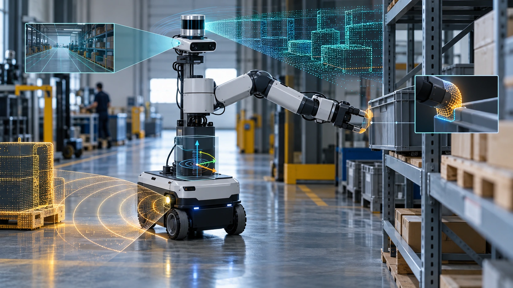
A warehouse robot approaches a pallet, a cobot reaches for a component, and an outdoor machine crosses a muddy yard. All three need to know where they are and what lies ahead. Yet the evidence they need arrives in different forms: reflected light, radio waves, acceleration, wheel rotation, motor current and contact force. The system design starts with a specific question: what must the robot know, by when, and with what confidence to act safely and productively?
A camera can distinguish a cardboard label from the pallet beneath it while offering no direct metric range from a single view. A laser scanner returns geometry with little inherent understanding of what an object means. An inertial unit reports rapid movement but accumulates position error if integrated alone. Joint encoders describe the robot’s own motion; they cannot prove that a gripper actually holds a slippery object. Each instrument supplies a partial observation of physical reality. A practical sensing architecture combines those observations with explicit assumptions about timing, calibration, environment and failure.
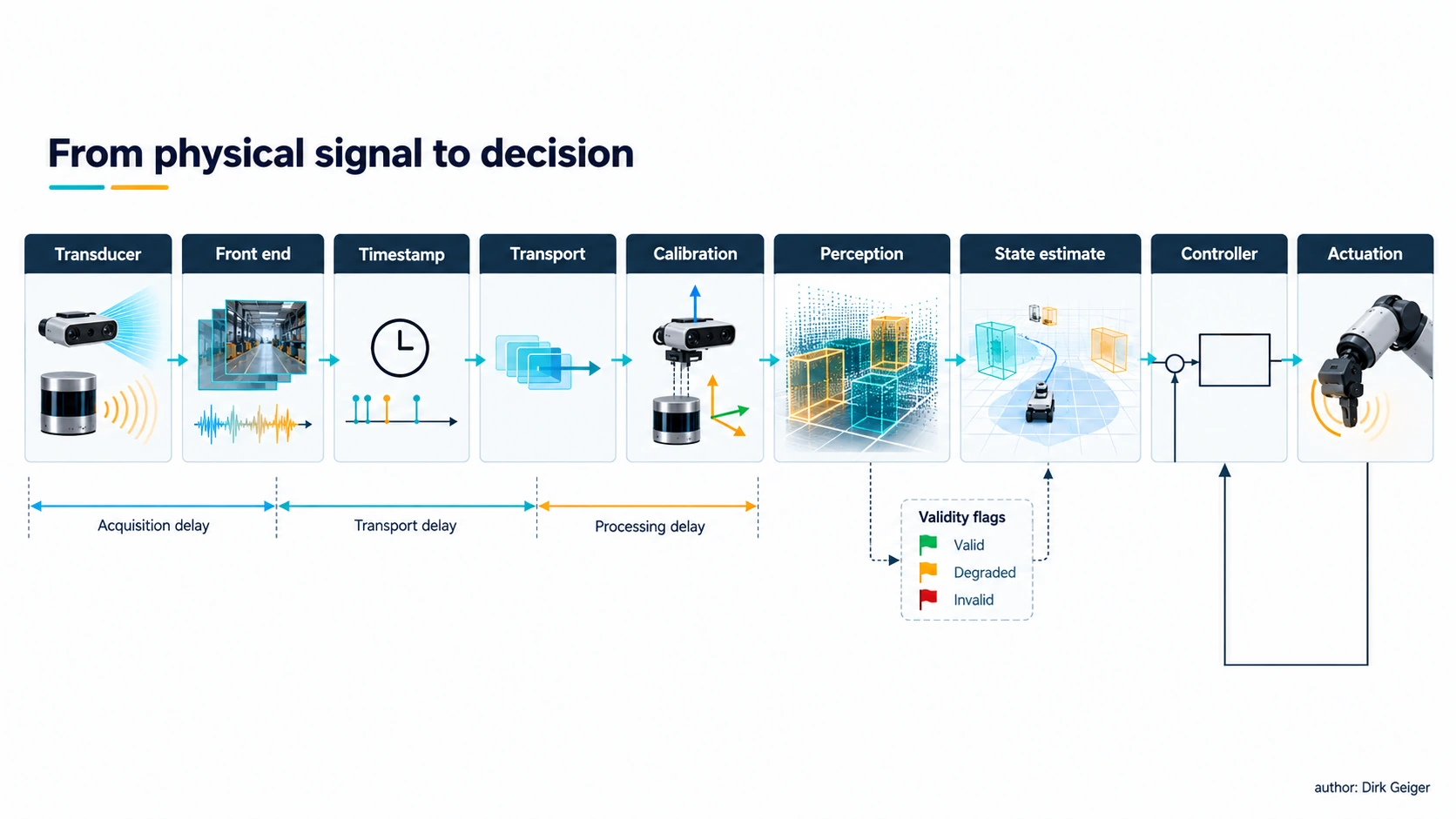
The word “sensor” also hides several layers of engineering. The transducer creates a signal; the analog front end and converter shape and digitize it; a timestamp locates the observation in time; a driver delivers data with units and validity; calibration maps it into a coordinate frame; perception turns measurements into estimates; and the controller decides whether the estimate is trustworthy enough for action. An attractive sensor specification can be defeated by a flexible mount, a dirty window, a saturated interface or a frame timestamp assigned after a long processing queue.
The requirement can be written as a decision contract. For a pallet approach, specify the obstacle classes and reachable volume, the maximum age of a position estimate, and the motion permitted when evidence becomes stale. A perception output then has an accountable consumer: navigation, manipulation or protective control. The same camera may contribute to several consumers, yet each needs its own acceptance threshold and fallback. This separation keeps a high-quality image from being mistaken for a complete answer to a safety question.
The sensing-stack figure follows one observation from the physical interface to action. At every handoff, units, clock domain, frame and validity must survive. A contact flag with no force direction, or a depth pixel without a calibrated pose, can be technically present and operationally unusable.
Cameras: detail, context and ambiguity
Visible-light cameras carry extraordinary semantic density. Texture, color, text, gestures, material boundaries and object identity can be inferred from images. A forward-facing camera helps an AMR read a scene; wrist cameras resolve alignment just before grasping; downward cameras can inspect floor markings or a hand’s contact region. Several cameras expand coverage and reduce occlusion, but each adds exposure control, data movement, synchronization and calibration work.
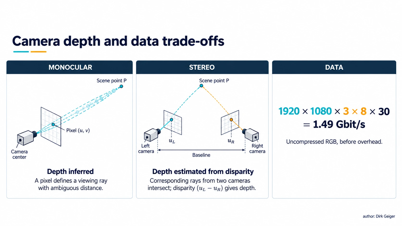
A monocular pixel identifies a viewing ray, not a unique distance. Stereo estimates disparity between corresponding features in two views; its depth uncertainty grows with range and weak texture. Structured light and time-of-flight depth cameras supply their own illumination and measured depth, with limits set by sunlight, reflections, multipath, working distance and competing emitters. Rolling-shutter readout can distort rapidly moving scenes; exposure choices that preserve a bright doorway may lose a dark aisle. Imaging quality must be checked against the actual illumination, motion and surfaces in the mission.
Intrinsic calibration accounts for focal geometry and distortion; extrinsic calibration defines the camera pose relative to the robot. OpenCV’s calibration documentation describes estimation of camera matrices, distortion and reprojection error [S1]. On a moving robot, a small angular mounting error projects into a large range error farther away. Temperature, vibration, impact or replacement of a bracket can change the answer after a factory calibration has passed. A calibration acceptance test therefore belongs to commissioning and service, with detectable drift where practical.
Image bandwidth grows with pixel count, bit depth and frame rate; compression reduces link load at the cost of latency, artifacts or compute. Raw 1920 × 1080 RGB at eight bits per channel and 30 frames per second is about 1.49 Gbit/s before transport overhead, a calculated upper-path example rather than a typical compressed stream. Engineers must budget peak bursts, memory copies and inference timing alongside average throughput. Often a low-resolution wide view continuously watches for hazards while a targeted high-resolution stream supports manipulation.
Optical design starts at the working distance. A wide lens sees more of a corridor but allocates fewer pixels to a small hazard; a narrow lens supports inspection while leaving gaps outside its field. Overlap between views can aid tracking and calibration, although the overlaps vanish when a person or carried load blocks a lens. Mounting height, protective glass, focus and lighting deserve the same attention as model accuracy. An inspection camera aimed at a fixed fixture can use controlled illumination; a navigating robot has to accommodate changing ambient light.
For moving platforms, exposure time, motion blur and rolling-shutter skew interact with speed. A classifier may retain a label while the geometry needed for a precise grasp has become unreliable. The vision-tradeoffs figure links depth method and deployment condition; the appropriate acceptance test uses the surfaces, speed and light transitions of the intended task.
Laser and optical ranging: geometry with conditions
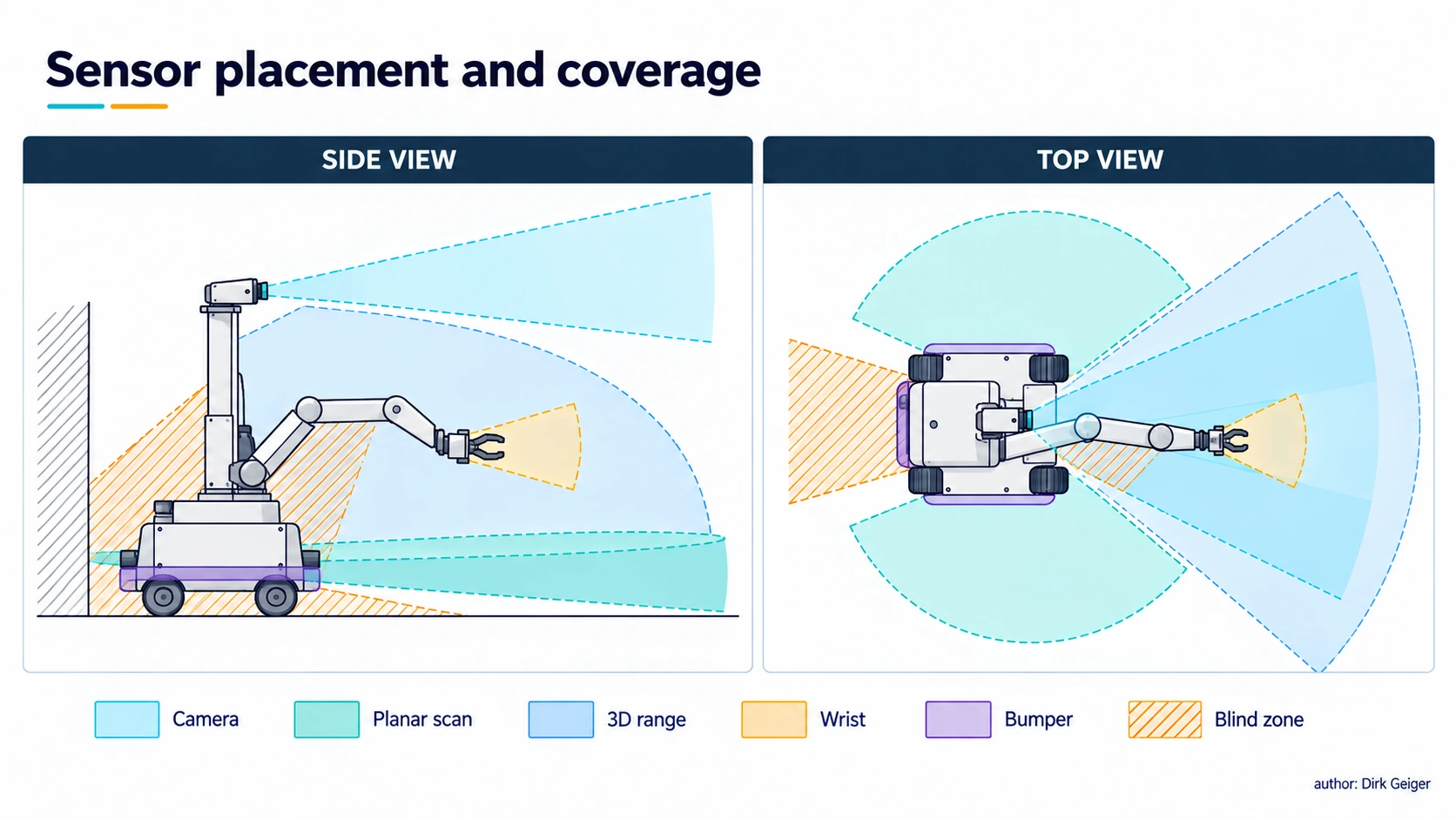
A two-dimensional laser scanner sweeps a plane and provides range versus angle. It is powerful for corridor localization and obstacle detection at a known height. A low scan can miss a protruding tabletop; a high scan can miss a small floor hazard. Three-dimensional LiDAR extends geometric coverage through a point cloud and supports mapping, localization and shape estimation, at higher acquisition, compute, power and integration cost. Range, angular resolution, reflectivity, update rate and coverage need to be evaluated as a system, not as isolated brochure maxima.
A laser return depends on surface reflectance and optical path. Glass, black materials, specular metal, direct sunlight, fog, rain, snow and dust can create missed or misleading returns. A survey of LiDAR perception in adverse weather describes scattering, occlusion, denoising and sensor fusion as active engineering concerns [S2]. Cleaning access and window contamination detection matter in a factory as much as a sophisticated perception model does. The measurement also has a precise acquisition time: a rotating scanner builds a “frame” over an interval while the robot and objects may be moving.
Short-range optical proximity sensors offer a different bargain. A small time-of-flight or reflective unit placed at a gripper, bumper or access panel can answer a narrowly defined question at modest data cost. Such sensors need material and geometry tests at their mounting location. Their field of view may include a robot’s own structure, and close-range crosstalk may look like a target. A few well-positioned local measurements can simplify control more than an additional panoramic sensor.
Coverage deserves a three-dimensional audit even when a navigation algorithm consumes a two-dimensional scan. The footprint of a sensor at one height says little about shelves above it, low objects beneath it or a load projecting beyond the robot base. The coverage figure shows how mounting and occlusion create blind zones. During a turn, stopping distance and swept geometry change; the detection volume should include the entire body and carried payload through the response interval.
A point cloud also needs a confidence model. Sparse returns around a dark or transparent object cannot be treated as free space merely because the surrounding wall is well observed. Maintain separate states for observed clear, observed occupied and unobserved. This distinction becomes especially valuable near dock openings, glass and rain-soaked surfaces.
Radar: useful evidence through difficult visibility
Radar measures radio-wave reflections and can estimate range and radial velocity; angular resolution and object separation depend strongly on aperture and processing. Its tolerance of darkness and some obscurants makes it useful for outdoor navigation and redundant detection. Camera–radar research describes their complementary information: image detail supports semantics, while radar contributes range and velocity cues [S3]. Radar data remain susceptible to multipath, clutter, metal-rich environments and ambiguous associations. A strong return is not automatically the object the robot intended to track.
Radar placement is an electromagnetic and mechanical problem. Radomes, nearby conductive parts, wheel housings and mounting angles alter patterns. Interference from other emitters and variations in the deployment site deserve trials. Radar can serve as an independent warning channel when an optical channel loses contrast, provided the two channels do not share a power, time, processor or contamination failure that defeats both. Its use for protective decisions still requires a safety case for the complete sensing and response chain.
Ultrasonic sensing can also cover close approaches with relatively small processing needs. Sound speed varies with temperature; absorbent, angled or small targets may return weak echoes, and multiple emitters may interfere. In a quiet indoor cell, ultrasonic sensing can be a useful local safeguard or docking aid. Outdoor wind, clutter and timing constraints can change that assessment. The right comparison is between the required detection envelope and measured performance, including the target’s least favorable orientation.
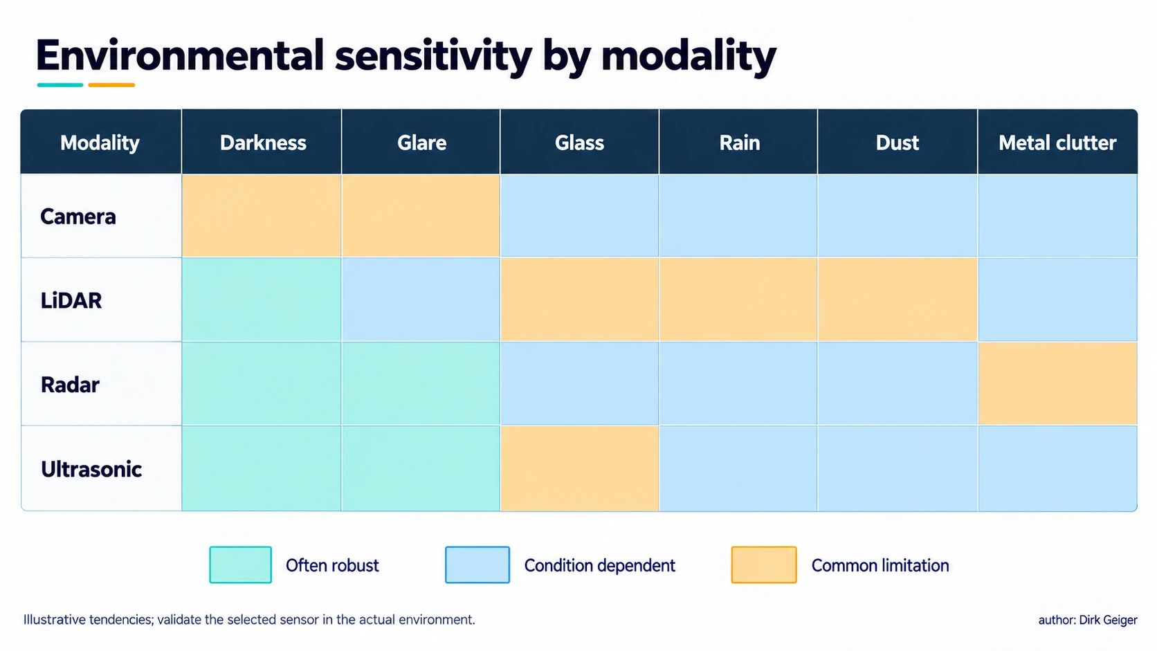
Radial velocity is a strong clue for an approaching object, yet tangential motion can produce little radial change. Radar tracks therefore depend on geometry and repeated observation. A person walking across the robot’s path and a stationary metal column may require different association logic even when their returns are initially close. The environment matrix captures where complementary modalities help; each cell is a test hypothesis for the site, not a guaranteed ranking.
Close-range acoustic sensing brings another timing problem: an echo may arrive from a previous pulse or another emitter. Pulse scheduling and cross-talk checks belong in the design when several units operate together. Both radar and ultrasound benefit from target sets that include the awkward cases: thin edges, soft materials, oblique surfaces and objects partly hidden by the robot’s own payload.
Proprioception: where the robot thinks its body is
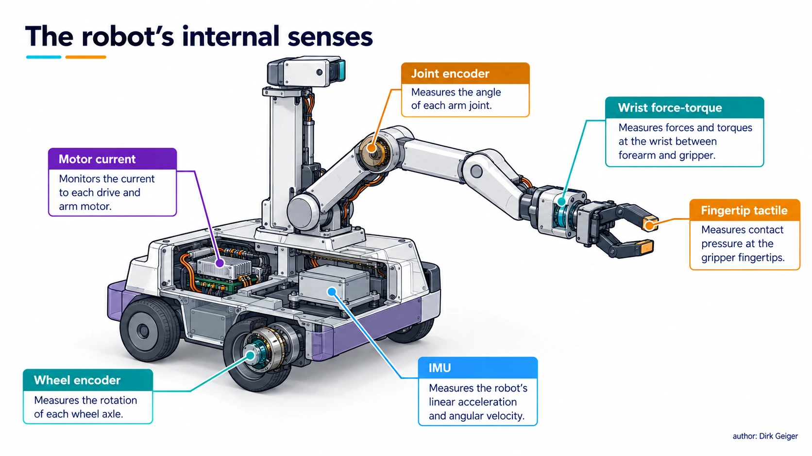
Encoders measure joint or wheel displacement; current and voltage measurements reveal aspects of actuator effort; inertial measurement units combine accelerometers and gyroscopes to track rapid motion. Together they form the robot’s sense of its own body. A wheel encoder can yield precise short-term travel on firm ground and a deeply wrong distance during slip. An inertial unit can bridge brief visual loss while gyro bias accumulates. A joint position can be known accurately while elastic transmission deflection leaves end-effector position less certain.
Mounting is consequential. An inertial unit on a vibrating motor housing sees disturbances different from those at the body center. Encoder readings need a clear definition of which side of the transmission is observed. Temperature drift, quantization, backlash and timestamp skew all appear in the state estimate. Contact sensors, force-torque sensors, torque estimators and tactile arrays close the loop between commanded movement and actual interaction. A gripper’s motor current may suggest contact, yet it also rises with friction or a mechanical jam. A tactile patch at the fingers can locate pressure and incipient slip, subject to wear, hysteresis and calibration.
The hand and foot need unusually local evidence. Force estimates from motor current are attractive where mass and wiring are constrained; they inherit uncertainties in torque constants, temperature and transmission friction. A six-axis wrist force-torque sensor provides a more direct interaction signal but needs overload protection and a clear coordinate transform. Distributed tactile sensing offers spatial contact information and creates packaging, multiplexing and repair challenges. In legged locomotion, ground contact classification and load distribution are time-critical because a mistaken support state can quickly become a balance problem.
Body sensing becomes more useful when it distinguishes commanded torque, electrical effort and measured external load. They are related through a drivetrain with losses, compliance and friction. A torque estimate that works in a warm, freely moving joint may shift after a cold start or a collision. For manipulation, contact detection should therefore be checked against the particular mechanical path and expected motion. At a foot, an incorrect contact transition changes the assumed support polygon and can invalidate the next control step.
The body-map figure places each observation near the physical quantity it constrains. A wheel encoder observes rotation at the axle; a wrist transducer observes load at its mounting plane; a fingertip array observes local pressure. Their transforms and mechanical offsets need explicit ownership so that a replacement hand or wheel module does not silently reuse an obsolete calibration.
Location comes from reconciling imperfect observations
Global navigation satellite systems support outdoor position estimation with sky visibility, but blockage, reflections and interference can weaken them around buildings or under cover. Ultra-wideband anchors, visual landmarks, LiDAR maps and wheel odometry can support indoor localization; each introduces installation and maintenance obligations. A facility map can drift operationally when racks move. An anchor can fail or be relocated. Localization confidence should change when the environment stops matching the assumptions under which it was built.
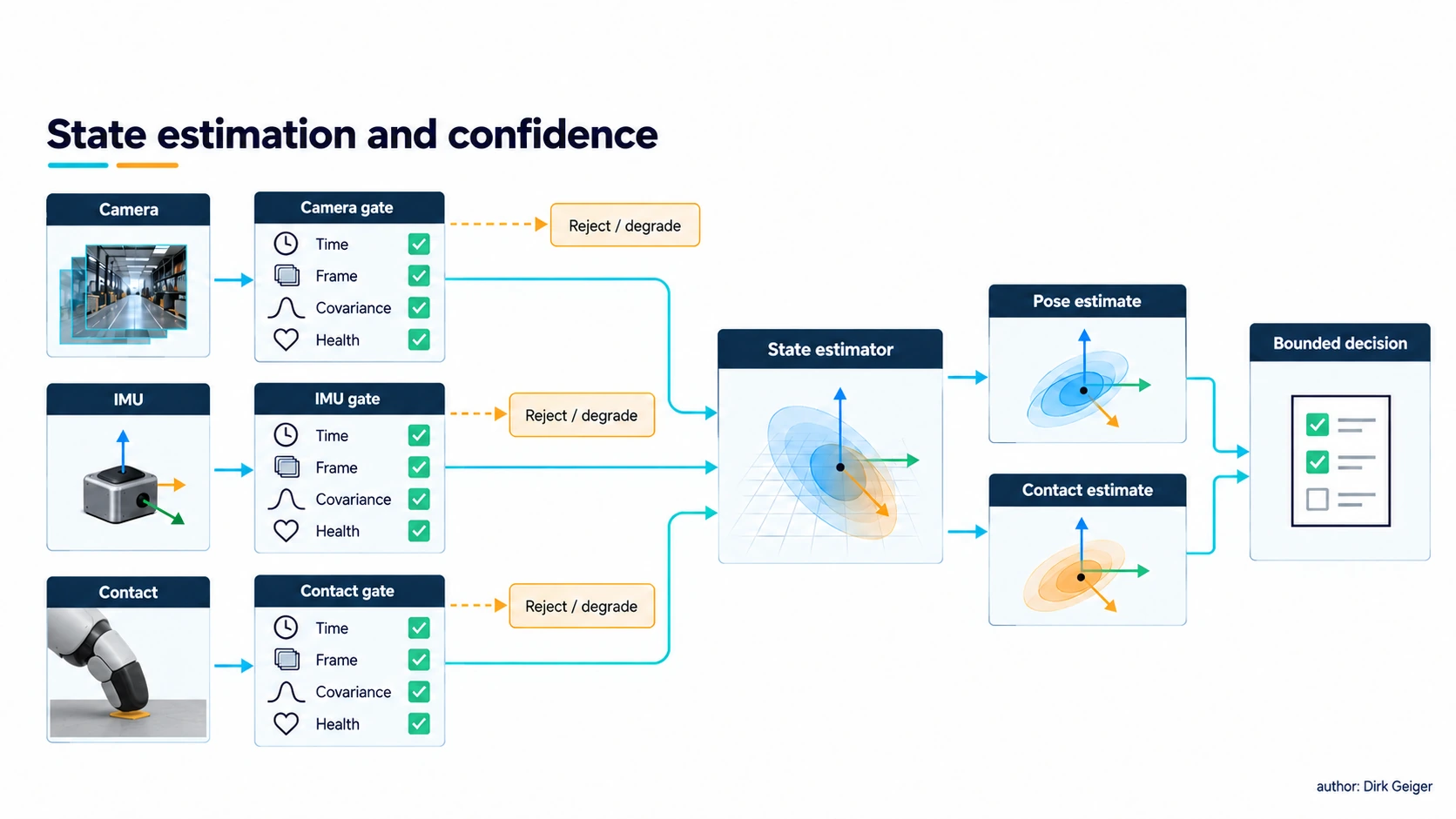
A state estimator combines measurements with a model of motion, uncertainty and observation quality. An extended Kalman filter, factor graph or other fusion method can be appropriate depending on dynamics, delay and compute resources. The essential discipline is more basic: use the acquisition timestamp, the correct coordinate transform and an uncertainty representation that reflects observed error. An estimator that reports a narrow covariance through a long occlusion may be numerically tidy and physically untrustworthy. Outlier rejection and innovation monitoring help expose inconsistent measurements, though correlated failures can still fool a fusion process.
A camera and an inertial unit can stabilize pose between image updates; wheel odometry can help in smooth corridors until traction changes; LiDAR geometry can correct accumulated drift when distinctive structures appear. Map updates, loop closures and recovery after losing position are operational functions. If localization uncertainty exceeds the envelope allowed for a maneuver, the controller should slow, request a better view, return to a landmark or enter a defined safe behavior. Confidence has value only when it changes the action.
The estimator’s uncertainty must remain connected to the decision envelope. A map match can appear persuasive in a repetitive aisle where several locations look alike. A single plausible association may pull the pose toward the wrong bay. Independent landmarks, motion consistency and recovery behavior matter as much as the nominal position error. The fusion-flow figure separates inputs, health gates and pose estimates before a bounded motion decision; a failed gate should alter what the controller may do.
Maps also age. A new rack layout can be a useful observation for a human and a confusing anomaly for a localization stack. Operational ownership should cover map changes, anchor surveys, sensor replacement and rollback. For a fleet, a change to shared geometry can affect many machines at once, so validation on a representative route should precede deployment across the site.
The clock is part of the measurement
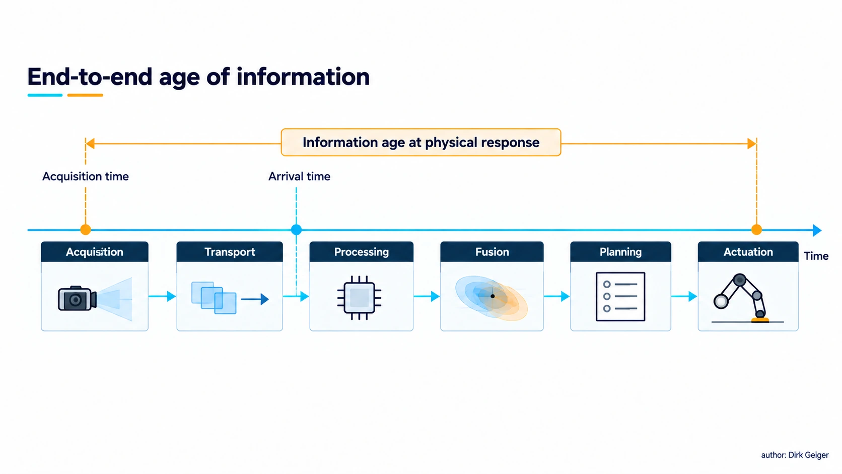
A timestamp means the instant a physical quantity was sampled, exposed or integrated, not simply when a software callback received it. A 50 ms mismatch at 1 m/s corresponds to 5 cm of travel before geometric and model errors are considered. A scanning sensor may need per-ray timing; an image exposure may span a nontrivial interval; a force sample may arrive after filtering. Joining these records by arrival order alone creates false alignment and can make a correct algorithm act on an impossible scene.
The sensing budget therefore follows a path: acquisition, front-end filtering, conversion, transport, decoding, inference, fusion, planning and actuation. End-to-end age matters more than a single sensor’s advertised sample rate. Buffers and compression may smooth bandwidth while quietly increasing age. A design should specify maximum permitted data age for each decision, tolerate occasional missing samples explicitly and measure worst-case behavior under concurrent compute and network load.
Synchronization methods range from shared triggers and local hardware counters to network clock protocols. Their achieved accuracy depends on implementation, topology and measurement; a protocol name alone supplies no guarantee. A robot can preserve a monotonic time base, record clock quality and reject observations after synchronization loss. When a remote model is involved, local obstacle handling and joint protection still need bounded response paths.
A latency allocation should distinguish average delay from tail delay. A stream that usually arrives in 20 ms can still fail a maneuver if rare bursts queue for much longer. Logs should carry the acquisition time, processing milestones and control consumption time, allowing the age of information to be reconstructed after an incident. The timing figure makes this distinction visible: a recently delivered estimate can describe a scene measured before the obstacle moved.
For a moving robot, timing error becomes spatial error. The 50 ms and 1 m/s example yields 5 cm of travel, but the resulting hazard margin also depends on braking, obstacle motion and uncertainty in the clock. Sampling faster has limited value if inference queues grow with input rate. A lower-rate path with bounded age may support a more dependable decision than a nominally faster path with unpredictable bursts.
Fusion needs independence and honesty
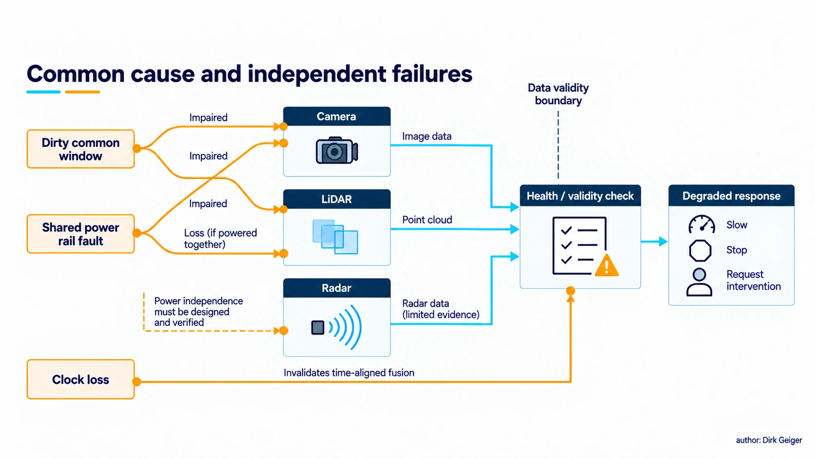
Complementary sensors improve a robot because their strengths cover different questions and their failure modes can sometimes be separated. Fusion is not a vote in which three weak estimates automatically beat one strong measurement. A camera and LiDAR looking through the same dirty window share a contamination fault. Two cameras powered from the same rail share a brownout. A radar and a camera with separate optics may still share a misleading map or an incorrect transform. A redundancy claim must trace the entire path from physical measurement to safe response.
A layered approach keeps raw health, object hypotheses and task decisions distinguishable. Early fusion can exploit pixel-to-point correspondences but demands precise calibration and synchronization. Later fusion lets modalities operate separately and reconcile detected objects, with possible loss of detail. Research on vision–radar fusion distinguishes several such design choices [S3]. The practical choice depends on available labeled data, failure detection, processor budget and the acceptable behavior when one stream disappears.
Each output needs a validity contract: measurement range, age, confidence, coordinate frame, calibration version and relevant fault flags. Faults should be injected during verification: cover the camera, heat the sensor, unplug a time source, swap a calibrated module, change floor traction and introduce reflective surfaces. A safe state may require controlled motion to stop or stabilize the robot. A missing stream is a meaningful input. Its allowed response should be defined before the first deployment.
Fault independence can be drawn as a graph of shared resources. Follow optics, cleaning system, rails, connectors, clocks, processing nodes and the model assumptions used to interpret the scene. The fault-path figure highlights several ways that apparently different measurements can fail together. Diversity becomes credible when the design can identify a fault and still execute the specified degraded behavior within its response budget.
Confidence calibration is equally important. A model score is often a ranking signal, while a control decision needs a relationship to missed detections under the relevant operating conditions. Test sets should separate routine scenes from rare but consequential ones, and report uncertainty in the regions where the robot will actually act. When association between radar and camera objects is ambiguous, preserving competing hypotheses for another observation may be safer than collapsing them prematurely into one confident track.
Selecting an architecture with real constraints
Sensor price is only the entry cost. The delivered system pays for mounts, windows, wiring, power conversion, interface capacity, compute, calibration fixtures, factory test, cleaning, replacement and field diagnostics. An extra camera can be inexpensive as a component and expensive as a validated stream. A more expensive sensor may simplify site preparation or shorten recovery from ambiguous scenes. Compare candidates through the mission’s detection envelope and lifetime service model.
| Modality | Strong evidence | Typical weakness | Integration burden |
|---|---|---|---|
| Camera | Appearance, labels, gestures | Lighting, occlusion, depth ambiguity | High data and inference; optical calibration |
| Depth camera | Local surface geometry | Range, sunlight, reflective surfaces | Moderate to high data; depth calibration |
| 2D/3D LiDAR | Metric range and geometry | Weather, transparent or weak returns | Scanning time, maps, optical maintenance |
| Radar | Range, radial motion in poor visibility | Clutter and coarse semantics | EM integration and association |
| IMU/encoders | Fast body motion and displacement | Drift, slip, bias | Timing and physical models |
| Force/tactile | Local interaction and contact | Wear, hysteresis, sparse coverage | Mechanical integration and calibration |
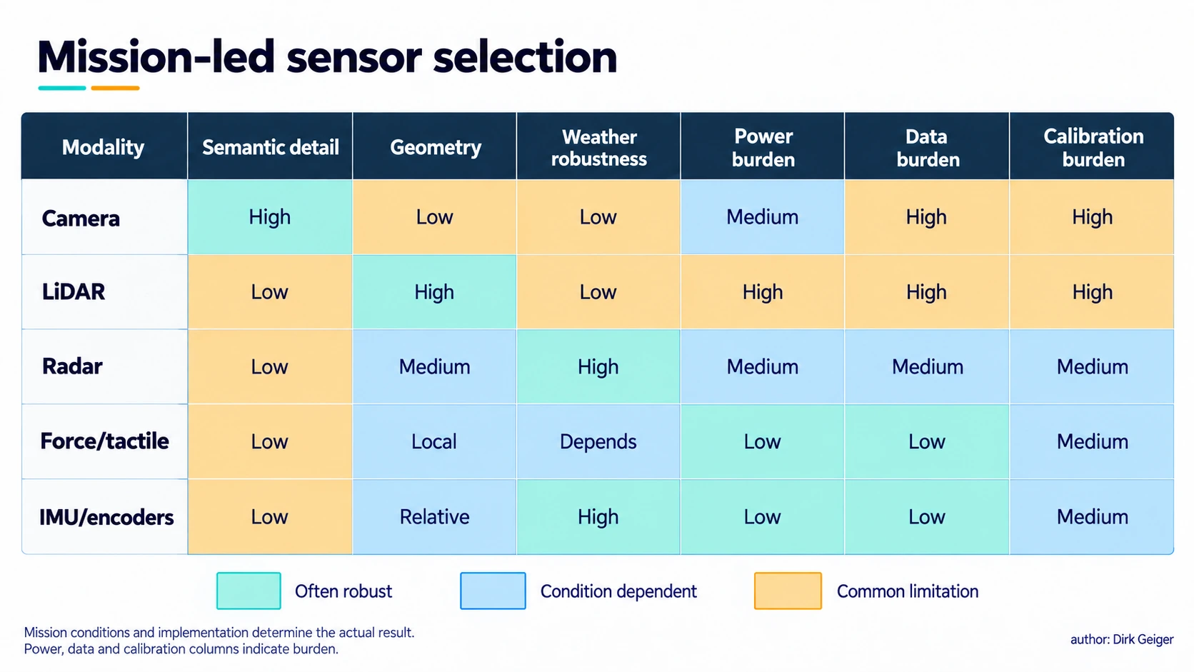
The table describes tendencies across device classes; each selected part needs its own measured operating envelope. Price, watts and processing load depend on the exact device, resolution, rate, enclosure and algorithm. Procurement comparisons should demand measured operating points: power at idle and full rate, data at the chosen encoding, detection probability across relevant targets, calibration time, recovery after fault, and maintenance labor. A weighted score can make a decision visible, but a hard safety or mission requirement should remain a gate rather than being averaged away by low cost.
Architecture selection is a constrained optimization, with some requirements acting as gates. For example, a sensing set that cannot cover a specified stopping volume is excluded before comparing purchase price. Remaining candidates can be assessed through power across operating states, compute headroom, network load at peak rate, calibration labor, repair time and environmental exposure. The selection chart visualizes these qualitative dimensions without turning site-dependent performance into an invented universal score.
Modularity helps only if interfaces preserve meaning. A replacement sensor needs an electrical and data interface, but also a defined coordinate frame, timestamp origin, calibration record and diagnostics. Otherwise, a seemingly compatible module can change the robot’s effective perception. Service procedures and versioned configuration are therefore part of the architecture cost.
Four missions, four sensible emphases
Indoor logistics. Predictable aisles, moving people and changing pallets reward dependable near-field obstacle detection, localization and docking. A common candidate combines wheel odometry and IMU with a planar scanner or depth sensing, plus cameras for labels and semantic context. Low protrusions, glass partitions and forks at unusual height require explicit coverage tests. Site maps, cleaning schedules and re-localization paths can dominate long-term availability.
Manufacturing. Precision and repeatability place calibration, controlled illumination and end-effector sensing at the center. Fixed cameras may be advantageous because the cell can provide rigid mounts and known geometry. Wrist vision and force sensing support insertion and contact-rich assembly. Protective sensing and collaborative operation need their own validated risk assessment. Robot perception used for quality inspection has different acceptance criteria from perception used to prevent hazardous contact.
Outdoor work. Sun, precipitation, dust, vibration and large changes in scale demand environmental qualification. GNSS can anchor broad position when usable; inertial, wheel or leg odometry bridge interruptions; cameras, LiDAR and radar contribute different scene evidence. Lens heating and cleaning, drainage, enclosure design and mud on the lower field of view are architectural concerns. Evaluation has to cover seasons and the rare conditions that set the robot’s operational boundary.
Human interaction. Facial direction, hand gesture, voice, proximity and contact can each inform intent, with uncertainty and privacy implications. Wide-area perception predicts approach; close-range sensors and force limits govern physical interaction. A robot should avoid treating a gesture classifier as consent for contact or a depth map as proof that a hand is clear. The safety response needs a measured stopping envelope, an uncertainty margin and a route for human intervention.
Across all four, there is no universal “sensor count.” The architecture changes with task speed, acceptable downtime, maintenance access and the consequence of a missed event. A modular core can reuse timing, health monitoring and interfaces while leaving room for a different optical head, radar placement or hand sensing where the mission justifies it.
Consider a warehouse robot carrying a load that obscures its forward camera. The navigation controller can continue only if another channel covers the swept path and localization remains valid. A deliberately defined reduced speed or stop state is more useful than a generic “sensor fault” alarm. At a docking station, a short-range sensor may take over the final centimeters while the broader navigation stack supervises the approach.
In a manipulation cell, the relevant uncertainty narrows from scene-wide location to contact geometry and force. An operator may move a fixture by a few millimeters and expose a calibration dependency that never appeared in empty-cell testing. A robot working outside faces a different change: rain can reduce optical returns at the same time as mud changes traction. Combining geometry with proprioception helps, provided the software recognizes that both channels have changed quality.
Prove the sensing chain in the field
A credible test plan begins with requirements expressed as observable events: detect a person entering a defined volume; identify a part before grasp; estimate contact force within an acceptable error band; localize sufficiently to pass a doorway. For each event, define operating conditions, detection and false-alarm criteria, latency, uncertainty and recovery behavior. Record the sensor configuration and software versions with the evidence. Bench performance does not transfer automatically to a vibrating machine in a busy site.
Test the limits deliberately. Change light levels and glare; introduce transparent, dark and reflective targets; vary weather and contamination; provoke wheel slip; obscure one view; induce clock offset; move a sensor by a small known angle. Evaluate the whole response, including stop distance and graceful degradation. Measurements at nominal conditions should be accompanied by distributions and worst-case trials, especially where a safety case depends on them.
Production and service complete the design. A factory needs repeatable calibration fixtures and acceptance limits; an operator needs diagnostics that distinguish a dirty window from a failing imager; a technician needs a replacement procedure that restores the coordinate transform. Logged data can reveal systematic misses and drift, subject to privacy, bandwidth and retention policy. When failures are made visible, the sensing architecture improves across a fleet instead of only inside a laboratory.
A robot’s senses become valuable at the moment a physical uncertainty changes a physical decision. The best architecture is the one that provides enough timely, calibrated and independent evidence for that decision, acknowledges the limits of every modality, and continues to behave coherently when the world refuses to match the test scene.
Evidence should be traceable from requirement to test result and field behavior. A test record can name the target, trajectory, environmental state, sensor health, software build and measured response time. Retain failures as first-class data: a missed detection with a reflective target explains more about deployment risk than hundreds of easy successes. Repeated trials estimate variability; fault injection shows whether alarms and degraded behavior occur when the decision is under load.
Monitoring continues after commissioning. Drift in calibration residuals, rising rates of rejected measurements, contaminated windows and unusual recovery frequency can signal a weakening sensing chain before a visible stop. Fleet logs need a policy for access, retention and privacy, especially when cameras observe people. A service action should close the loop with a new acceptance test, so repair restores measured performance rather than merely clearing the alarm.